Updated: Jan 20, 2022
Not everyone is destined to be a data analyst, or an Excel sheets guru, but I most working professionals have to use Excel or Google Sheets. Think of it like Maths; you may detest it, and you still don’t know why you had to find x, but at the very least, you need to know how to count all those bands you be stackin’.
I want to give you baseline competency that will make you less of a liar on your resumé. Here are a few features and/or functions you should know (and use).
First, let’s clarify the difference between a function and a formula in Google Sheets. Functions are pre-made formulas and you might have seen them before: SUM, MAX, MIN, IF, VLOOK UP etc. Place an equal sign inside a cell and type any letter—the options you see are examples of functions. A formula, on the other hand, is an expression created by you to solve a specific problem. For example, adding figures using the plus (+) sign.
Formulas can include functions but functions cannot include formulas.
The expression below shows a formula that uses the IF function to define a pass mark.
=IF(B2>90,"PASS","FAIL")
TODAY is the most basic DateTime function you should know. Imagine you have an event coming up and you want to have a countdown showing how many days are left to the big day—place the Event date in one cell, today’s date in another cell by using =TODAY(), and create a third cell showing the difference between the 2 dates. TODAY() will update automatically daily. Below is an illustration:

If you want to review other DateTime functions, there’s a post for that here.
If you have a list of names in a column in “Firstname Lastname” format, and you want to place the first names and last names in separate columns, SPLIT would solve this in seconds.
For a more detailed walkthrough of SPLIT, there’s a post for that here.
⚠️: SPLIT is only available in Google Sheets, but Excel has several ways of handling this problem and this article covers them.
The main text functions: LEFT, RIGHT, MID, and FIND are useful for extracting parts of a text. LEFT returns specified characters from the extreme left of a text while RIGHT returns specified characters from the extreme right of a text. MID extracts a small chunk of text from a larger text, and FIND finds any character you’re looking for in a text and returns its character index or location.
The input shows the original text, the output shows the final product, and the last column can illustrates the “how”
⚠️: Every character in a text string has an index. Think of an index as the address or position of a character. Even spaces, commas, asterisks, etc are characters. The first character has index 1. For example, in the name John Doe, “J” has an index of 1 and the space has an index of 5.
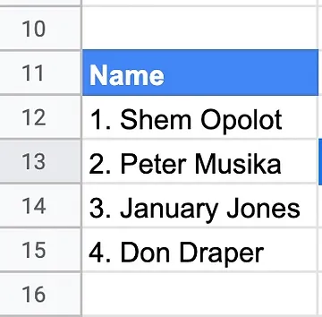
Text functions can be useful if you are trying to generate unique user IDs for event attendees from a list—you may want to use the first letter or the first name plus the last 4 digits of the phone number. OR, you may want to clean up an error in a column—if a name list comes with numbers before every name as shown below, you can use LEFT to remove the numbers. Can you use the LEFT function to remove the numbers, periods and spaces before the names?
Pivot tables will help you summarise large data quickly. Imagine you have the data in the table below:
Here’s a preview of the data for the TL;DR folks:
What would you do if your manager asked you which regions had the greatest revenue? It would take you ages to manually identify the number of unique regions and then add up each region’s corresponding revenue totals. However, with pivot tables, this process takes less than 5 seconds. If you want a quick walkthrough of pivot tables, I got you.
⚠️: In Google Sheets, you can find pivot tables in Insert in the toolbar. The interface is slightly different from Excel but intuitive once you understand the concept.
COUNTIFS lets you count the number of values that meet a specific criterion, while SUMIFS lets you add up all the values that meet a specific criterion.
The syntax for both is similar:
COUNTIFS: =COUNTIFS(criteria_range1, criterion1, [criterion_range2], [criterion2],....)
SUMIFS: =SUMIFS(sum_range, criteria_range1, criterion1, [criterion_range2], [criterion2],...)
In the illustration below, we have grades (Pass/Fail/None) and we want to know how many passed, failed or were ungraded. We also want to know the individual total score of those that passed, failed or were ungraded respectively.
⚠️: COUNTIFS and SUMIFS do the same thing as COUNTIF and SUMIF; however, the former accepts multiple criteria and therefore renders the latter redundant. [Some small small use of former and latter there to make sure you’ve had your coffee 😅]
IMPORTRANGE allows you to copy live data from one sheet to another sheet or workbook.
Why not just copy and paste? Well, IMPORTRANGE will automatically update the data in the new sheet when the data in the old sheet is updated. Copy and paste wishes it could 🧨.
When would you use IMPORTRANGE? When you create a survey via Google Forms, the responses are automatically stored in a Google Sheet. What if you want to use the sheet with responses to perform additional operations? Say, you want to add additional columns to capture attendance or completion of some assignment. Rule #1 of dealing with data is to NEVER TAMPER WITH THE RAW DATA. IMPORTRANGE takes 2 arguments—the link to the original sheet and the range of cells you want to import—both of which should be surrounded by double quotation marks.
IMPORTRANGE(spreadsheet_url, range_string)
⚠️: The range_string must include the sheet name with an exclamation mark at the end—this is standard notation; I don’t make the rules—and the range of cells. For example, “Your Sheetname!A1:D1000”.
When you import a range of data, always highlight the cell where the formula is entered. Deleting the contents of this cell will omit the data instantly.
The final formula would look as follows ⬇️
=IMPORTRANGE("https://docs.google.com/spreadsheets/d/get_your_own_sheet_link", "Your Sheet name!A1:I1000")
There are many more functions and features in Google Sheets you could use. Full disclosure: I started this point with 2 features and it ballooned uncontrollably to 6. We could add scrollable tables in Google Sheets and charts as well, but you don’t want to spend the rest of your life reading this blog. These 6 features will not make you an expert, but they will empower you to tackle most of the challenges you encounter daily in your spreadsheets.
Have a great week and don’t forget to subscribe if you want to get more content like this hot off the press!