Hi friend! This week we tackle a real work problem I encounter a lot.
You are preparing for a luncheon to launch your new product called Sobar. Sobar is a bar of soap that cures alcohol-induced hangovers by using it when you shower. Yep! TO THE MOON!! In preparation for the luncheon, you send out a google form to get the details of the attendees and get preorders of Sobar.
Make a copy of this Google Form and follow along.
The responses to a Google Form survey can be extracted to a Google Sheet and stored in your Google Drive. However, I often get the responses in a Google Sheet but find that I have to add more columns to clean up the data or make it more lucid. For example, in our hypothetical, we know the number of Sobars each attendee wants to order, but we need to compute their total bills. Here’s what we do:
First, we fill out the Google Form twice to get 2 responses to test in our spreadsheet. We do this by previewing the form, filling it out and hitting submit.

Clicking the eye at the top right will preview the form
After submitting the 2 responses, we extract them into a google spreadsheet.

Click the spreadsheet icon, follow the prompts and create the spreadsheet
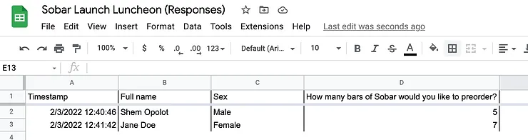
The Responses spreadsheet with our 2 responses
Google Forms does not let us build order forms without using add-ons. In a future post, I will show you how to use an add-on to create order forms and invoice clients automatically. However, today we must use the spreadsheet to compute the total amount to bill the attendees. Let’s say each Sobar costs UGX 50,000. We can compute the Total owed by multiplying the number of orders by 50000 in an adjacent column.
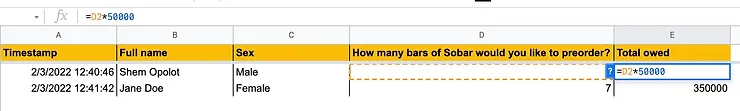
Calculate total owed by multiplying orders in the D column by 50000
We can also copy this calculation throughout column E to apply it to future responses. We do this by editing the formula to reflect a range and copying the formula downwards. We can specify the range: D2:D100; however, I usually just use the whole column (D2:D) to be safe. After all, sales are going TO THE MOON, remember?
The calculation is pretty simple but we have 2 problems:
Remember the first rule of working with data? “DO NOT EDIT THE RAW DATASET!”
Google Sheets does not make it easy for you to calculate in the original sheet and this is a good thing.
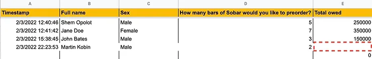
Notice the gap highlighted in red
But what should we do?
I talked about the IMPORTRANGE function a while back and we have a chance to use it. We use IMPORTRANGE to create a live copy of the original dataset. Every time we get a new response, the response is added to the original sheet and the copy we made using IMPORTRANGE.
We open a new sheet and set it up as shown below. Do not be intimidated or confused by the formatting; I just like pretty spreadsheets. However, I always place the link to the original spreadsheet at the top in cell A1, so I can access it quickly. In cell A2, I place a note that indicates where I am going to type my IMPORTRANGE function. This way no one (including future me) deletes the contents of cell A3 (labelled Timestamp), which will delete the whole imported range.
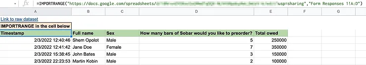
While clicking in cell A3, my IMPORTRANGE formula is shown in the formula bar
IMPORTRANGE takes 2 arguments: the link to the original spreadsheet and the sheet name, followed by an exclamation mark, and the columns you would like to import.
=IMPORTRANGE("Link_to_original_spreadsheet","Sheet_name!A:D"
With a copy of the original dataset, we can now add the Total owed column again and recalculate. However, this time we will use the ARRAYFORMULA function.
The ARRAYFORMULA function saves you time on repetitive calculations by automating them. The ARRAYFORMULA function has complex applications, but today, we will do something simple: Type the formula for calculating the total owed in the first cell below Total owed. Do not forget to add the range (D4:D) so that the calculation applies to all the numbers in column D. The formula should look something like this: D4:D*50000 depending on how your spreadsheet is set up. Before clicking ENTER to calculate, surround the formula in brackets (or parentheses, depending on the primary school you went to) and add ARRAYFORMULA in front of the first bracket (clearly we know the primary school I went to😅). Another way to activate ARRAYFORMULA is to click inside the formula bar and press Ctrl + Shift + Enter (Command + Shift + Return on Mac). ARRAYFORMULA will appear around the formula automatically.
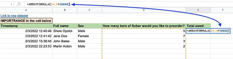
Your sheet should look something like this
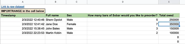
Now you can press ENTER. The calculations are made but the trailing zeros persist. Let’s ignore them for now.
To ensure the calculations will update automatically in this sheet when we get new responses, we return to the Google Form and submit another response. To ensure we are on the same page, enter a male called “Jake Kawesa” who preordered 10 Sobars.
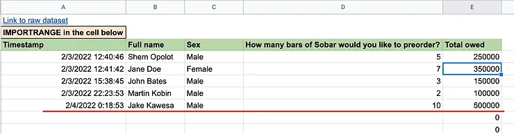
Would you look at our boy, Jake😁
We have solved problem #2! The calculations are updating automatically now.
Now that the calculations are automated, we could stop here. However, I’d like to remove the trailing zeros so the sheet looks neater.
First, it is important to understand why the zeros are showing up. We have used an array formula to perform a calculation on ALL the cells in column D. When the cell in column D is empty, 50000 is multiplied by the 0 in column D to give the zeros we see in column E.
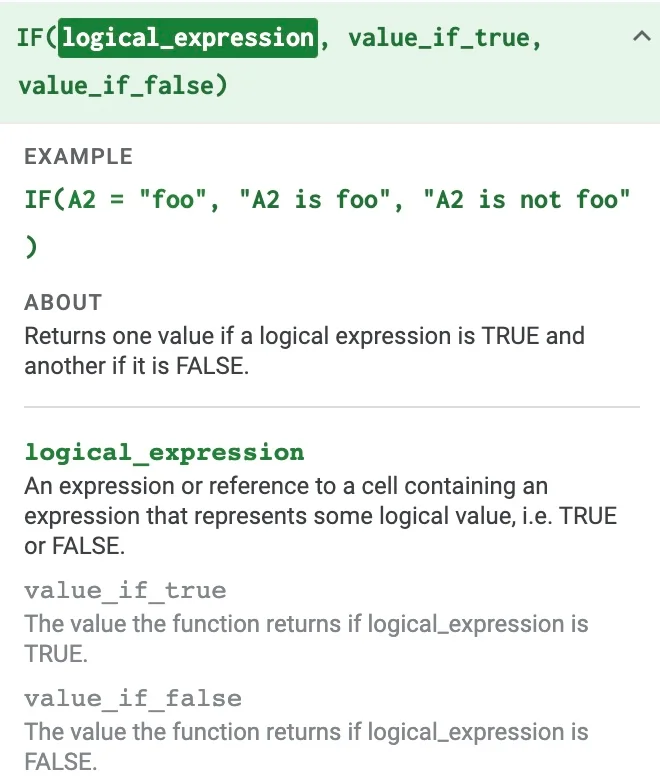
Using an IF function nested inside the ARRAYFORMULA function, we can tell Google Sheets to ignore the empty cells in column D so that the zeros disappear. Let me write it in words first then I’ll type up the formula:
We are going to tell Google Sheets to check inside column D, and look for entries. IF the cell is not empty, the calculation we want should be performed. However, IF the cell is empty, we want it to return an empty cell.
We will do this within the ARRAYFORMULA function so that the condition applies to all the cells in column D. We edit our array formula as follows:
=ARRAYFORMULA(IF(ISBLANK(D4:D),,D4:D*50000))
💡: In the formula above:
1. ISBLANK(D4:D) is the condition we check for in the IF function. ISBLANK checks if a cell is empty and returns TRUE or FALSE.
2. IF returns nothing if our condition (ISBLANK(D4:D) is TRUE, and it returns the result of our calculation (D4:D*50000) if the condition is FALSE. Here’s how to use IF:
If zeros persist, seek medical advice
The persistent zeros are gone and our sheet will update as new responses come in. Problem #1 solved!
Before you throw a dance party, I recommend you hide (not delete) the original sheet of responses so you are never tempted to mess with it.
The bible advises you to flee from temptation
This week’s post was quite involved but practical, I hope. Learning about the existence of cool functions is useless if you cannot use them to solve your daily problems. I hope this makes you excited to send out a survey.
Have a great week!