Updated: Apr 18, 2022
Hi friend! This week, I want to talk about special tables in Excel. Stop me if you heard this one before: have you ever looked at a colourful Excel spreadsheet and wondered why anyone would use so much colour so frivolously on a simple table? Well, there are 2 reasons for that I can think of:
When doing raw data entry in Excel, the data is seemingly in tabular form, but Excel does not recognize the data as a table. Excel treats the data as a range across cells. While this may seem inconsequential, there are many benefits to converting your data from the default range to a formatted Excel table, and that is what we are doing today.
YouTube video:
Excel workbook for practice:
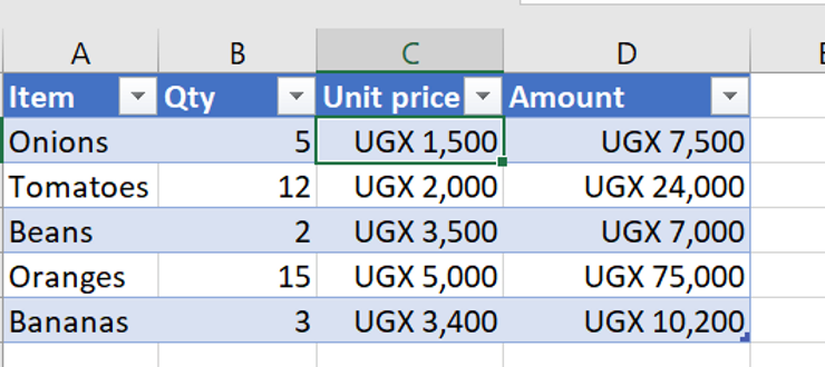
You have a grocery list and you want to add up the items in Excel to get your final bill before you head to the market. Let’s fabricate a grocery list real quick:
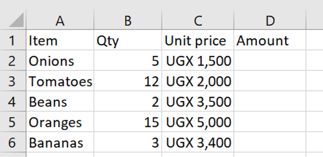
Orange you wondering why I like oranges?
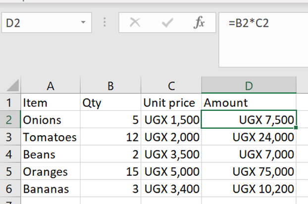
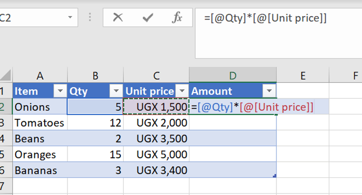
To get our overall bill, we can be basic and calculate the total amount to be spent on Onions and then copy the formula downwards (If you do not remember how to copy the formula downwards, check here; Hint: black cross in the corner of the cell). We find the total amount spent on Onions by placing an equal sign in cell D2, then multiplying the Quantity in B2 by the Unit price in C2.
The problem with the above method is if we forgot to add chicken to the list and want to update the list, we have to keep copying the formula downwards again to find the total by item and eventually, the overall bill.
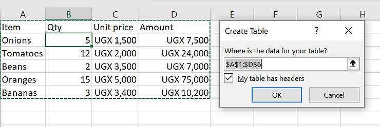
The faster way is to tell Excel to recognize the range of data from A1:D6 AS A TABLE. To do this, click anywhere in the range of data and hold Ctrl + T (or Command + T on a Mac). Green crawling ants dart around the range of data and a Create Table window pulls up. In the Create Table window, we leave the box that says “My table has headers” checked (this allows Excel to treat the first row as a header row, which is what we want), and click OK.
Our multicolored table has been created as shown below. You may not like the way it looks (and we can change that by clicking anywhere in the table and going up to Design or Table Design in your toolbar depending on your version of Excel), but you will love what it can do.
Let’s take our new table for a spin. Delete all the entries in the Amount column by selecting all the entries in the column and pressing Delete. Now, re-perform our earlier calculation to find the total price of Onions in cell D2 again (=B2*C2) and press enter. Do not worry about the new notation Excel uses; nothing has changed really. Do you see what happens? When in table form, Excel looks at your table and assumes you want to perform the same calculation throughout the column and does it for you.
Don’t be intimidated by the formula; the calculation stays the same
Once in table form, if we want to add any items we may have forgotten, we type in the row immediately below the last row in the table and Excel will include that entry in the table.
Let’s add 2 whole chickens, each costing UGX 30,000 and see what happens. The table updates with a new complete row for Chicken.
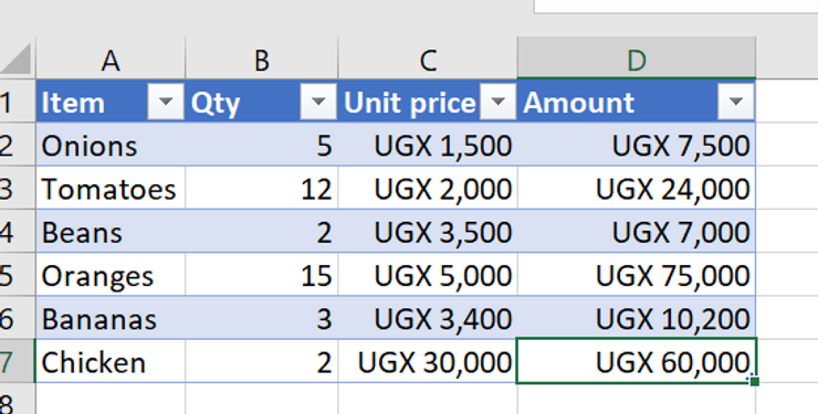
A complete row for the chicken is added to the Table automatically
What if we want to add the grand total for all the items? There are multiple ways to do this, but let’s do 2:
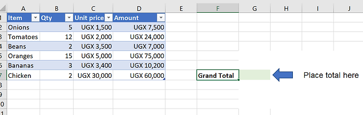
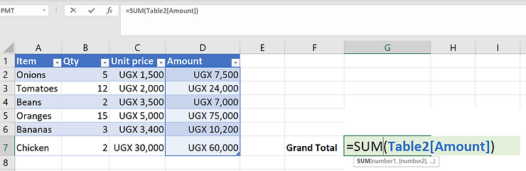
#2 (Continued): We want to enter the grand total in the shaded box above. However, while in table format, we can ensure that if any item is added to our grocery list, the Grand Total will update automatically. To do that, type the SUM function in the shaded box and open the bracket. Instead of selecting the range of cells from D2:D7, hover the cursor at the top of cell D1 where “Amount” is written until you see a downward-facing black arrow. Once you see the arrow, click the cell and press ENTER. Excel selects all the entries in the Amount column, our favourite crawling ants return, and we have our Grand Total in the shaded box. By using this method, you are telling Excel to include all current and future entries in the Amount column in your SUM function.
To test this, let’s add 5 Apples at UGX 5,000 each to the list and observe what happens to our Grand Total.
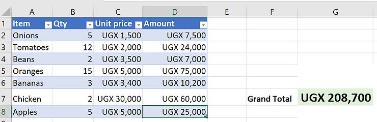
Adding Apples automatically raises the Grand Total
The above feature can be useful when you are managing income and expenses for your business in separate sheets. As long as you convert all the ranges to tables, you can automate the calculation of your Gross Profit in a third sheet by getting the Total Expenses in one sheet and subtracting them from the Total Income in another sheet. Try this on your own.
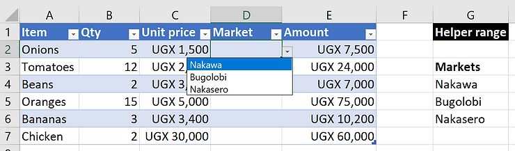
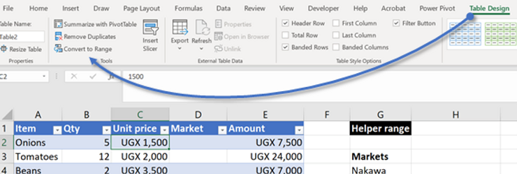
We visit 3 markets regularly: Nakawa, Nakasero and Bugolobi. What if we want to include a column showing which market we got the individual items from? (I know it doesn’t make sense, but don’t let logic get in the way of a good story) We add a column to our grocery list table called Market and use data validation to create a dropdown list of the 3 markets. If you don’t know how to create dropdown lists, submit my name for a Nobel prize here. For this particular dropdown list, we use a helper range of the Market names to create it. Remember, if you put the helper range in the column immediately next to the table, Excel will include it in our table, and we don’t want that.
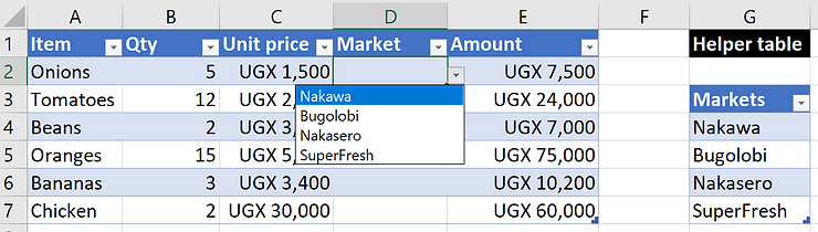
What if we find a new market called SuperFresh that sells more organic and more pretentious fruits and vegetables? We can’t resist; we must indulge. Tables in Excel allow us to update our dropdown list(s) automatically. We click in the helper range, convert it to a table, by pressing Ctrl + T (delete the word “Helper table” otherwise Excel will add it to the new table, OR simply edit the table range to exclude it) and follow the same process as before. Once in a table, add SuperFresh below Nakasero, and then check the dropdown in our original table. Voilà!
As much as tables are great, you may not always want the automation they provide. To convert the data back to a range, click anywhere in the table, go up to Table Design in the toolbar and then select Convert to Range. Excel will ask you if you’re sure about this life choice—be confident and click OK.
More often than not, you should convert your data in Excel to tables. They ensure new entries are updated automatically. If you create a chart with data from a table, when you update the table, the chart will update automatically. This is how you create basic dashboards. When creating pivot tables, placing the source data in a table will update the pivot table details as data entry continues. Don’t table tables for later, start using them now.
See you next time, and don’t forget to remove the chicken from the fridge before mum gets home.
PS: YouTube video resources
1. The file for the recent YouTube video is below
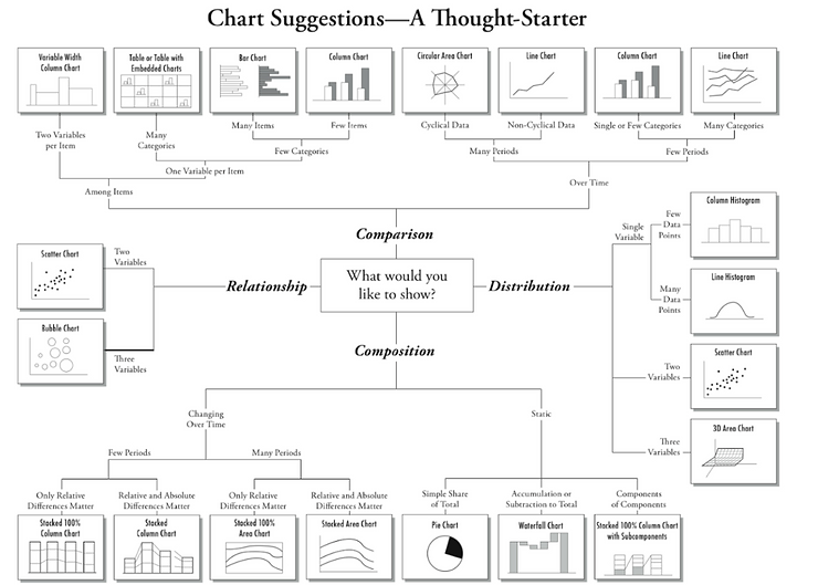
2. Which chart should you use?