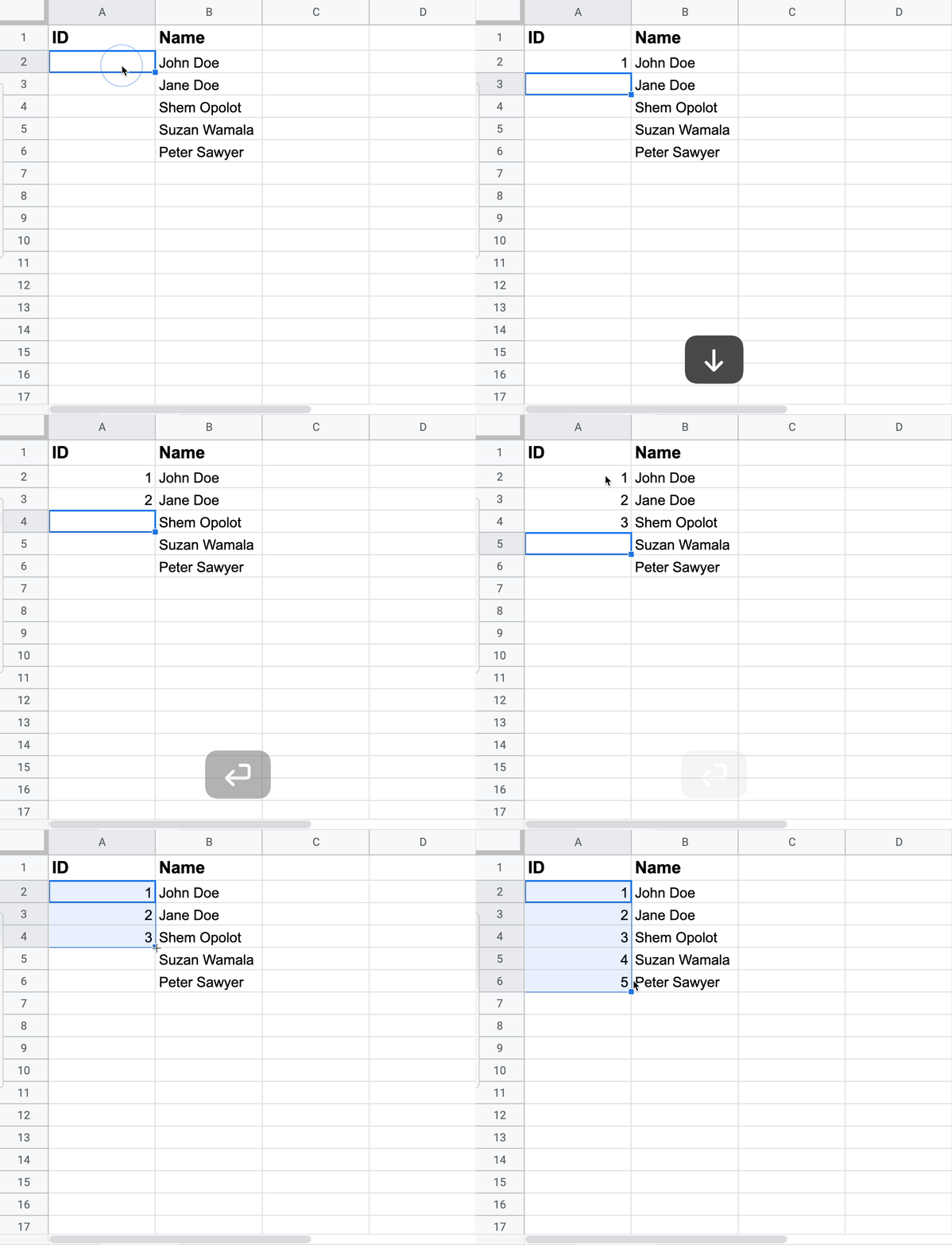
You’re creating a list of your favorite people and you want to assign a number to each person. How would you do it?
Like this?

You’re cute, but NO!
If your answer to that question was yes, please stick around for 2 more minutes. If you said no, stick around for my charm 😅.
While the method above gets the job done; especially, if the list is short and you have no friends, we can do better. You can do better. I am going to show you a way you can use the SEQUENCE function in Excel or Google Sheets to automate numbering your lists.
Let’s get into it 😎.
Here’s the video for this week ⬇️
The SEQUENCE function is great for generating random sets of numbers with one formula. I talked about it in this article if you want a crash course.

In this illustration, I generate a list of 10 numbers, starting from 1 and skipping every 3 figures
COUNTA counts all the non-blank cells in any selection. If the cell has anything in it (and I mean ANYTHING), count on COUNTA to count it.

Notice that I highlight cells A15 and A16 as well, but COUNTA returns a count of 14
We will combine these 2 functions to assign a number (ID) to every name on our list

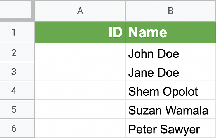
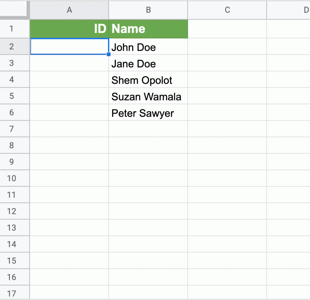
Our glorious list of faves 🥰
We will start with SEQUENCE and insert the COUNTA expression in the rows argument. The rows argument in the SEQUENCE function tells Excel how many rows of numbers you want to create, OR, how long you want your list to be. However, we may not know how many more names will be added to our list, so we use COUNTA instead of a specific number of rows and count all the non-blank entries in the entire name column (denoted by B2:B in the COUNTA expression). jjjbbbbb

I love my new screen capture tool!
Let us see our formula in action ⬇️

Every time you add a new name, a number is added automatically 🎉
I bet you can’t wait to make a new list! While you’re on Cloud 9, check out this article and learn how to make a cool to-do list in Google Sheets.
Have a good week ✌🏾.
